BForStrain Strain Rate Inversion Code
![]()
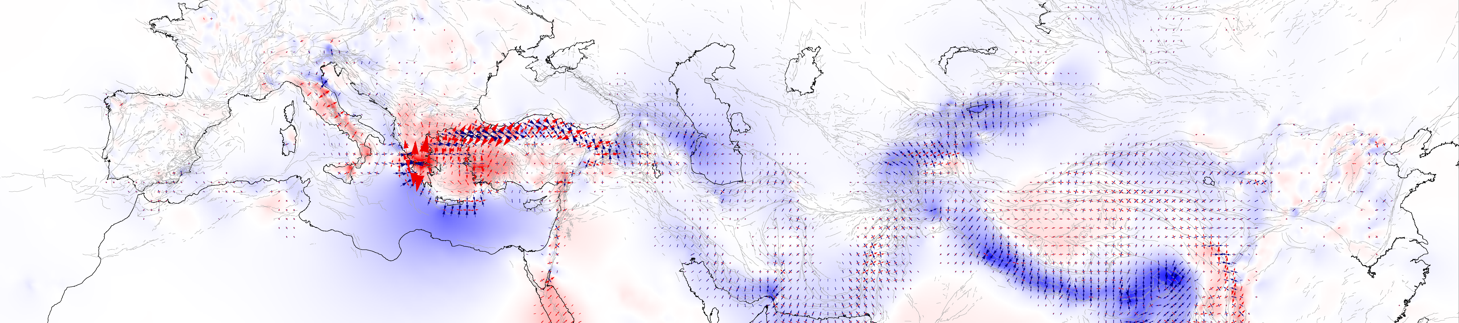
These codes compute strain rates on a trianglular 2D mesh using a geodetic velocity field. Body-forces in a thin elastic plate are used to compute a velocity and strain rate field computed at the centroids of the triangles in the mesh. The inversion solves for the distribution of body forces (at the triangle nodes) that best-fits the geodetic velocity field. You can specify a range of smoothing values (called beta) that minimize the magnitude of the body forces. There is also an optional second step that further minimizes strain rates below a specified threshold.
Parameters can be specified in params.py. The data used in Johnson (2024) from Zeng (2022) is currently loaded, along with creeping fault traces from the 2023 US National Seismic Hazard Model.
To run the demo, use the code below to download the repository and initialize a new environment
git clone https://github.com/jhdorsett/BforStrain
cd BforStrain
conda env create -f environment.yml
conda activate BforStrain
Then the code can be executed with the data provided using run.ipynb.
Project structure:
BforStrain
   | bForStrain.py
   |   |-- Mesh
   |   |   |-- create_gps_obs
   |   |   |-- create_creeping_segs
   |   |   |-- create_creeping_segs
   |   |   |-- crop
   |   |   |-- save
   |   |   |-- plotting_functions
   |   |   |-- coordinate_transforms
   |   |-- Inversion
   |   |   |-- bodyforce_greens_functions
   |   |   |-- creeping_greens_functions
   |   |   |-- prepare_inversion
   |   |   |-- invert
   |   |   |-- generate_uncertainty
   |   |   |-- post_process_results
   | disloc3d.py
   |   |-- dc3d
   |   |-- dc3d_wrapper
   | mesh2d.py
   |   |-- smooth2d
   |   |-- helper_functions
   | tools.py
   |   |-- helper_functions
   | data/
   |   |-- geodetic veolcities
   |   |-- creeping faults
   |   |-- coastline data (plotting)
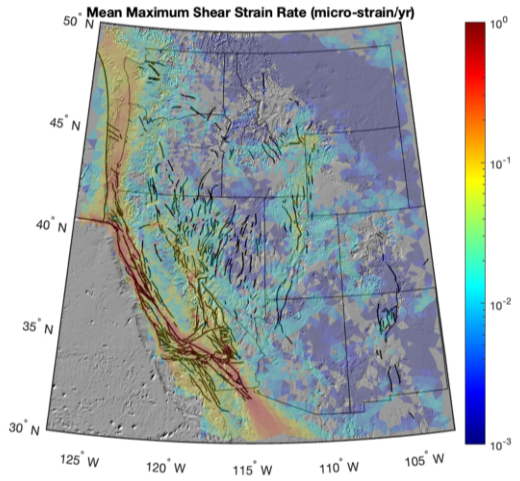
Here is a particular model realization generated using the western US geodetic data and fault configuration. The mesh is colored by max shear strain rate in each triangle. Geodetic observations and modeled velocities are shown as vectors, where each data point is the average of all GPS stations in that triangle.
This model is displaying the mean values for a suite run with three different damping parameters:
\[{\chi}^2_{( {\beta}=35)} = 1.91 \\ {\chi}^2_{( {\beta}=40)} = 2.05 \\ {\chi}^2_{( {\beta}=45)} = 2.18\]Including pseudo-velocity data (some offshore vectors).